3 Study area and data
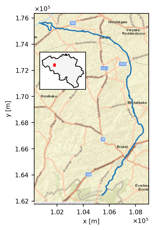
For these exercises, a hydrological dataset of the Zwalm catchment will be used. The Zwalm catchment is located in the centre of Belgium and can be considered a medium-scale catchment. Its main tributary, the Zwalmbeek, is visualised in Figure 3.1. During the period 2009-2025, a dataset of daily precipitation, potential evapotranspiration and discharge is at your disposal (see Section 3.3 for more information). The average annual rainfall and potential evapotranspiration of the catchment are 783 mm and 561 mm respectively, typical values for Belgium.
As mentioned in Chapter 2, all the processed data is available at data/processed. If interested, you can inspect (and execute) all downloading and processing steps yourself by following the instructions in scripts/data_download/README.md and scripts/data_process/README.md of the repository.
In the next section, more information is given on the data sources and processing steps for the different types of provided data. Note that all geographic data is provided in the Belgian Lambert 72 (BD72, EPSG:31370) coordinate reference system (CRS).
3.1 Catchment data
The data in the data/processed/catchment_info folder contains information on the river network and the catchment boundaries in the broad vicinity of the Zwalm catchment. The source of the river network is the Vlaamse Hydrografische Atlas (Vlaamse Milieumaatschappij 2026). The catchment boundaries come from the Oppervlaktewaterlichamen en hun afstroomgebieden, 2022-2027 dataset (Vlaamse Milieumaatschappij 2023). In Chapter 4, you will be asked to delineate the catchment boundary of the Zwalmbeek yourself. The provided catchment boundaries can be used for comparison. Both files are provided as ESRI Shapefiles, called afstroomgebied.shp and vlaamse_hydrografische_atlas.shp respectively.
3.2 Digital terrain model
For the catchment delineation of Chapter 4, a digital terrain model (DTM) is provided in data/processed/digital_terrain_model. This DTM is derived from the Digitaal Hoogtemodel Vlaanderen II DTM at 1m spatial resolution (Agentschap Digitaal Vlaanderen 2014). To reduce the size of the dataset and speed up the computation, the DTM has been resampled to a spatial resolution of 10.0 m by averaging. The DTM is provided as a GeoTIFF file, called DHMVII_DTM_1m_upscaled_10m.tif.
3.3 Meteorological and discharge data
Both meteorological forcings and observed discharge are provided in the folder data/processed/forcings_discharge. All this data is retrieved from Waterinfo, a website which combines hydro(meteorological) data from both the Flanders Environment Agency and Flanders Hydraulics Research. Programmatic access to the data is possible via the Python package pywaterinfo, as demonstrated (for your information only) in scripts/data_download/waterinfo_download.py.
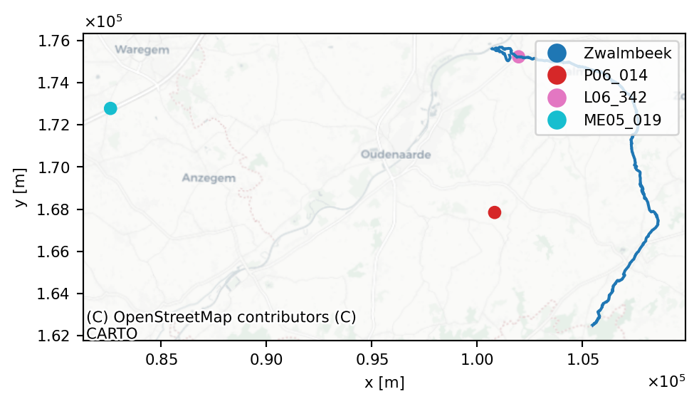
The combined forcings and discharge dataset is provided in the CSV file forcings_discharge.csv. An overview of the the original data sources is given in Table 3.1. Note that mm is equivalent to mm/d because of the daily time resolution. The locations of the different measurement stations are additionally shown in Figure 3.2. Some processing details:
- Precipitation (\(P\)) is the areal average of four rain gauges (Elst, Maarke-Kerkem, Zingem and Ronse) using Thiessen polygons as weighting factors1, clipped to the Zwalm catchment as delineated by the Flemish government. When a gauge has no data for a given day, the Thiessen weights are recomputed with the remaining gauges. The Thiessen weights for each gauge when all gauges are available, are given in Table 3.1.
- Potential evapotranspiration (\(E_\mathrm{p}\)) is estimated using the Penman equation at a meteorological station. Missing values are gapfilled with the daily, smoothed climatology of \(E_\mathrm{p}\). Smoothing occurs by applying a moving average with a centred window of 11 days.
- River discharge (\(Q\)) is measured near the mouth of the Zwalmbeek in the village of Nederzwalm. No gapfilling is applied to this variable, as it is only used for model evaluation, not as a model input.
| Variable | Units | Station | Station ID | Thiessen weight |
|---|---|---|---|---|
| Precipitation | mm | Elst OTT_P | plu06a-1066 | 0.74 |
| Precipitation | mm | Maarke-Kerkem_P | P06_014 | 0.09 |
| Precipitation | mm | Zingem_P | P06_040 | 0.17 |
| Precipitation | mm | Ronse OTT_P | plu12a-1066 | 0 |
| Potential Evapotranspiration | mm | Waregem_ME | ME05_019 | |
| River Discharge | m³/s | Nederzwalm/Zwalmbeek | L06_342 | |
| Precipitation of catchment | mm | Nederzwalm/Zwalmbeek | L06_342 |
Consequently, following columns are present in forcings_discharge.csv:
['',
 'precipitation',
 'potential_evapotranspiration',
 'river_discharge',
 'precipitation_vmm_catchment']
Note that the first column without a name is the index column, which contains the date. The column precipitation_vmm_catchment is an alternative catchment precipitation product of the Flanders Environment Agency (Precipitation of catchment in Table 3.1), gapfilled with the Maarke-Kerkem gauge. It is only provided for comparison, for what follows use precipitation.
The correct interpretation of the date is that the data value corresponds to the daily sum (\(P\) and \(E_\mathrm{p}\)) or daily mean (\(Q\)) of the day indicated by the date. For example, the value of \(P\) on 2020-01-01 corresponds to the total precipitation that fell during that day.
Tip
To read in forcings_discharge.csv, checkout the documentation for pandas.read_csv(), specifically of the index_col and parse_dates parameters, to correctly read in the dataset.
3.4 Satellite soil moisture
In Chapter 8, the goal is to improve the hydrological model predictions by assimilating observations of soil moisture. Here, we’ll use satellite-derived surface soil moisture (\(SSM\)), which is provided in the folder data/processed/satellite_soil_moisture.
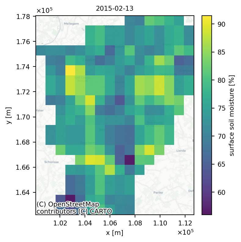
The original data source is the SSM product at 1 km spatial resolution over Europe from the Copernicus Land Monitoring Service (European Union’s Copernicus Land Monitoring Service 2026). An example of the original data for one example date is shown in Figure 3.3. The \(SSM\) values are expressed in percent saturation and are representative of the top few centimetres (~5cm) of the soil.
For ease of use, the dataset has been processed to a timeseries by taking the average \(SSM\) value over the Zwalm catchment and subsequently removing outliers. The resulting final timeseries is called satellite_soil_moisture.csv, which has following columns:
['time', 'ssm', 'noise']with time the date of acquisition, ssm the spatially averaged \(SSM\) and noise is the spatially averaged standard deviation of the \(SSM\) following a simple mean2.
See the Hydrology course in the Bachelor for more information on this technique↩︎
Alternatively, one could follow the rules of propagation of uncertainty. In that case, any function \(f\), the standard deviation is given by \(\sigma_{f}={\sqrt {\left({\frac {\partial f}{\partial x}}\right)^{2}\sigma_{x}^{2}+\left({\frac {\partial f}{\partial y}}\right)^{2}\sigma_{y}^{2}+\left({\frac {\partial f}{\partial z}}\right)^{2}\sigma_{z}^{2}+\cdots }}\) assuming no covariance between \(x,y,z\cdots\) and linearly approximating \(f\). Note that an average is a linear function, so here this is not an approximation. With the average \(\bar{x} = \frac{1}{N} \sum_{i=1}^N x_i\) as \(f\), \(\frac{\partial f}{\partial x_i} = \frac1N\) and so \(\sigma^2_{\bar{x}} =\sum_{i=1}^N \left(\frac{\partial \bar{x}}{\partial x_i} \right)^2\sigma_i^2 = \frac{1}{N^2} \sum_{i=1}^N \sigma_i^2\). This assumption of no covariance is a strong one however, which does not necessarily hold up for soil moisture retrievals which exhibit spatial correlation. Therefore, we make the safe assumption of perfectly correlated pixels, which increases the estimated uncertainty to \(\sigma_{\bar{x}}^2 = \frac{1}{N} \sum_{i=1}^N \sigma_i^2\)↩︎